Simple Demo

Welcome

Please note that this is not a Python tutorial. We assume that you are aware of basic Python coding and concepts including the use of conda and pip. If you did not install mesh2scattering already please do so by running the command

pip install mesh2scattering[examples]

The [examples] dependency installs additional dependencies, which are required to execute this notebook.

Note that this notebook do the same as the demo.py, so its up to you what you prefer.

After this go to your Python editor of choice and import mesh2scattering

import mesh2scattering as m2s
import pyfar as pf
import spharpy
import os
import numpy as np
import matplotlib.pyplot as plt
import trimesh

create the project

we need to set the paths for the meshes. First for the sample and then for the reference plate. Please notice that the sample should lay on the x-y-plane where z is the hight.

sample_path = os.path.join('meshes', 'sine_n10_1', 'sample.stl')
reference_path = os.path.join('meshes', 'reference_n10_1', 'sample.stl')
project_path = os.path.join(os.getcwd(), 'project')
if not os.path.isdir(project_path):
    os.mkdir(project_path)

Define the frequency array. For simplicity we just use 3 frequencies. If you want to create 3rd- or 1st octave band frequencies have a look on pyfar.dsp.filter.fractional_octave_frequencies.

frequencies = np.array([1000, 2000, 3000, 4000])

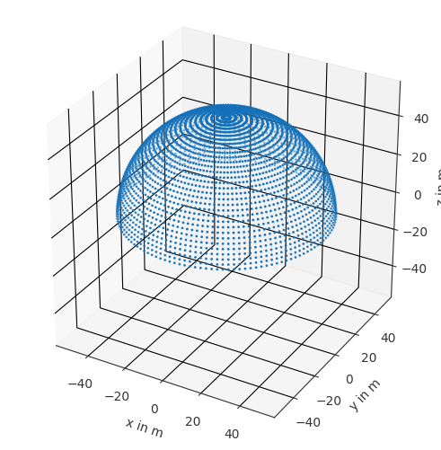
Now we need to define the source and receiver positions. Therefore we create a sampling grid, including the pole and removing the lower part of the grid.

receiver_radius = 50
receiverPoints = spharpy.samplings.gaussian(
    n_max=63, radius=receiver_radius)
receiverPoints = receiverPoints[receiverPoints.colatitude < np.pi/2]
receiverPoints.show()
plt.show()

The receiver positions can now go into its related class. The class requires faces, but they can be simply calcualted by the class by using from_spherical.

evaluation_grid = m2s.input.EvaluationGrid.from_spherical(
    receiverPoints, 'grid')

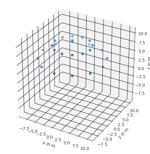
Same for the source positions. The radius is set to 10 according to the diffusion ISO Standard 17497-2.

source_delta_deg = 30
source_radius = 10
sourcePoints = spharpy.samplings.equal_angle(
    source_delta_deg, source_radius)
sourcePoints.weights = spharpy.samplings.calculate_sampling_weights(
    sourcePoints)
sourcePoints = sourcePoints[sourcePoints.colatitude < np.pi/2]
sourcePoints.show()
plt.show()

Now we need to set the parameters of the sample.

structural_wavelength = 0.177/2.5
sample_diameter = 0.8
model_scale = 2.5
sample_baseplate_hight = 0.01

Furthermore we need to define the symmetry properties of the sample. In our case we have a sine-shaped surface, so the sample is symmetrical to the x-axe and y-axe, therefore we set the symmetry_azimuth to 90 and 180 degree. A rotational symmetry is not give, so we set it to False.

symmetry_azimuth = [90, 180]
symmetry_rotational = False

Lets collect all the metadata of the sample and the surface into the related class object. The meta data will not influence the simulation or postprocessing, they are just collected and exported in the sofa file at the end.

sine_description = m2s.input.SurfaceDescription(
    structural_wavelength_x=.177/2.5,
    structural_wavelength_y=0,
    structural_depth=.051/2.5,
    surface_type=m2s.input.SurfaceType.PERIODIC,
    symmetry_azimuth=symmetry_azimuth,
    symmetry_rotational=symmetry_rotational,
)
mesh_sine = m2s.input.SampleMesh(
    mesh=trimesh.load(sample_path),
    surface_description=sine_description,
    sample_baseplate_hight=0.01,
    sample_diameter=sample_diameter,
    sample_shape=m2s.input.SampleShape.ROUND,
)
reference_description = m2s.input.SurfaceDescription(
    structural_wavelength_x=0,
    structural_wavelength_y=0,
    structural_depth=0,
    surface_type=m2s.input.SurfaceType.FLAT,
    symmetry_azimuth=[],
    symmetry_rotational=True,
)
mesh_reference = m2s.input.SampleMesh(
    mesh=trimesh.load(reference_path),
    surface_description=reference_description,
    sample_baseplate_hight=0.01,
    sample_diameter=sample_diameter,
    sample_shape=m2s.input.SampleShape.ROUND,
)

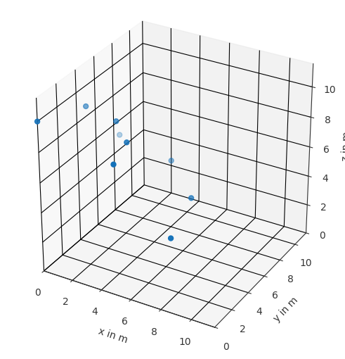
This symmetry settings are required for the postprocessing and and we can speed up our simulating by skipping incident angles and calculate them in the postprocessing by mirroring the existing data. Therefore we can skip the azimuth angles grater than 90 degree for the source positions.

sourcePoints_reduced = sourcePoints[sourcePoints.azimuth <= np.pi/2]
sourcePoints_reduced.show()
plt.show()

Now we can add put the source positions into the correct class formate. We will define Plane waves.

sourcePoints_reduced.cartesian *= -1
sound_sources = m2s.input.SoundSource(
    source_coordinates=sourcePoints_reduced,
    source_type=m2s.input.SoundSourceType.PLANE_WAVE,
)

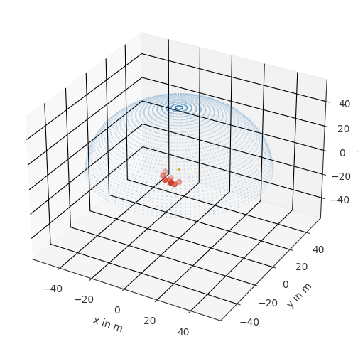
let’s plot the scene

sample = trimesh.load_mesh(sample_path).vertices
sample_coords = pf.Coordinates(sample[:, 0],sample[:, 1],sample[:, 2])
ax = pf.plot.scatter(receiverPoints, s=1/20)
pf.plot.scatter(sourcePoints_reduced, ax=ax)
pf.plot.scatter(sample_coords, ax=ax, s=1/72)
plt.show()

Now we can create the project. Please notice that the project was already created and simulated for demo.

m2s.input.write_scattering_project_numcalc(
    project_path=os.path.join(project_path, 'sine'),
    project_title='sine',
    frequencies=frequencies,
    sound_sources=sound_sources,
    evaluation_grids=[evaluation_grid],
    sample_mesh=mesh_sine,
    )
m2s.input.write_scattering_project_numcalc(
    project_path=os.path.join(project_path, 'reference'),
    project_title='reference',
    frequencies=frequencies,
    sound_sources=sound_sources,
    evaluation_grids=[evaluation_grid],
    sample_mesh=mesh_reference,
    )

run project

To execute the project you need to build the NumCalc project. If you use Windows, the exe can be directly downloaded and on mac or linux it can be build, see the function documentation for more information.

numcalc_path = m2s.numcalc.build_or_fetch_numcalc()

Now we can run the simulation, this may take some time. This example is already simulated so we don’t need to wait. If we don’t explicitly define then numcalc_path it will use m2s.numcalc.build_or_fetch_numcalc() in the background to determine the numcalc_path.

m2s.numcalc.manage_numcalc(
    os.path.join(os.getcwd(), project_path), wait_time=1)

Starting manage_numcalc with the following arguments [Apr 02 2026, 09:31:09]
----------------------------------------------------------------------------
project_path: /Users/anne/git/_pyfar/Mesh2scattering/examples/project
numcalc_path: /Users/anne/git/_pyfar/Mesh2scattering/mesh2scattering/numcalc/bin/NumCalc
max_ram_load: 16.00 GB (16.00 GB detected, 4.52 GB available)
ram_safety_factor: 1.05
max_cpu_load: 90 %
max_instances: 8 (8 cores detected)
wait_time: 1 seconds
starting_order: alternate
confirm_errors: False


Per project summary of instances that will be run
-------------------------------------------------
Detected 2 NumCalc projects in
/Users/anne/git/_pyfar/Mesh2scattering/examples/project


'sine' is already complete
'reference' is already complete


... waiting for the last NumCalc instances to finish (checking every second, Apr 02 2026, 09:31:09)

All NumCalc projects finished at Apr 02 2026, 09:31:09

Post processing

Now we need to create the scattering pattern sofa files out of the simulation results. Here the symmetry is also applied. since the reference sample is always rotational symmetric, the data for the missing angles are rotated in this was sample and reference data will have the same dimensions and coordinate

m2s.output.write_pressure(os.path.join(project_path, 'sine'))
m2s.output.write_pressure(os.path.join(project_path, 'reference'))

 Writing the project report ...

 Writing the project report ...

calculate the scattering coefficient for each incident angle and the random one from the scattering pattern

m2s.process.calculate_scattering(
    os.path.join(project_path, 'sine_grid.pressure.sofa'),
    os.path.join(project_path, 'reference_grid.pressure.sofa'),
    'sine',
    )

SOFA file contained custom entries
----------------------------------
OriginalFrequencies, RealScaleFrequencies, Lbyl, SampleStructuralWavelength, SampleStructuralWavelengthX, SampleStructuralWavelengthY, SampleModelScale, SampleDiameter, SpeedOfSound, DensityOfMedium, ReceiverWeights, SourceWeights, SampleSymmetryAzimuth, SampleSymmetryRotational
SOFA file contained custom entries
----------------------------------
OriginalFrequencies, RealScaleFrequencies, Lbyl, SampleStructuralWavelength, SampleStructuralWavelengthX, SampleStructuralWavelengthY, SampleModelScale, SampleDiameter, SpeedOfSound, DensityOfMedium, ReceiverWeights, SourceWeights, SampleSymmetryAzimuth, SampleSymmetryRotational

Read and plot data

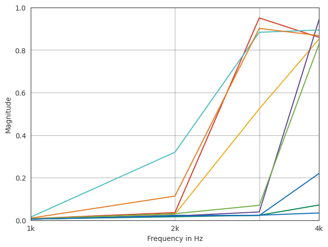
example of plotting the scattering coefficient

s_rand_path = os.path.join(
    project_path, 'sine.scattering.sofa')

s_rand, _, _ = pf.io.read_sofa(s_rand_path)
ax = pf.plot.freq(s_rand, dB=False)
ax.set_ylim(0,1)
plt.show()

SOFA file contained custom entries
----------------------------------
OriginalFrequencies, RealScaleFrequencies, Lbyl, SampleStructuralWavelength, SampleStructuralWavelengthX, SampleStructuralWavelengthY, SampleModelScale, SampleDiameter, SpeedOfSound, DensityOfMedium, ReceiverWeights, SourceWeights, SampleSymmetryAzimuth, SampleSymmetryRotational